Machine Learning Classification with RapidMiner

A short introduction of the dataset

We picked the dataset on spamming by sms. It consisted of 5572 rows of data and with two columns one being the SMS message and the other depicting if the message was spam or ham. 13% of the messages were marked as spam. It consisted of different types of messages, some being very short and others longer with some being very legible, meanwhile others consisted mostly of weird symbols.

The data cleaning process and its result

The first step for cleaning our data was to remove unwanted things from the dataset. This includes duplicates or irrelevant data.

The first thing that we checked was if we have any missing values. Our dataset did not have any missing values so we did not have to replace anything.

We started with 5572 rows of data and after deleting duplicates we ended up having 5169 rows of data.

After that we deleted irrelevant data from our dataset. This included some symbols from the data: . We also decided to remove a phrase that was used often but would not give us any valuable information: <#&gt.

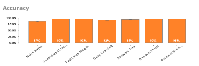
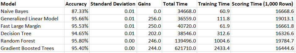
Comparing different Machine Learning algorithms with the dataset.

Models we chose to generate:
Naive Bayes
Generalized Linear Model
Fast Large Margin
Deep learning
Decision Tree
Random Forest
Gradient Boosted Trees

The accuracy of results was very high and we got an overview of the total time it took for the algorithms to train and score the dataset.

Process
We Imported the dataset to Rapidminer and changer column v1 to label because we want to know if an email is considered spam or ham.

Looked over the statistics of imported data to see if there are any missing values. No missing values were detected.

Since we did not need to change any of the data the only thing we did was to rename the columns. v1 changed to Content and v2 changed to Spam or ham.

After that we started the Auto model. Selected task was to predict if an email is spam or ham. Prepared targets showed that 4,516 was marked as ham and 653 was marked as spam in the given dataset.

After that we selected the inputs as v2 so ham or spam.

Process graph

The results that were obtained

We ran the algorithms and got following grading results:
Naive Bayes – spam 9%, ham 91%
Generalized Linear Model – spam 33%, ham 67%
Fast Large Margin – spam 17%, ham 83%
Deep learning – spam 1%, ham 99%
Decision Tree – spam 4%, ham 96%
Random Forest – spam 11%, ham 89%
Gradient Boosted Trees – spam 10% 90%

Naive Bayes 

Naive Bayes is an algorithm for predictive modeling. It is a high-bias, low-variance classifier, and it can build a good model even with a small data set. Typical use cases involve text categorization, including spam detection, sentiment analysis, and recommender systems.

In our data set naive bayes predicted that about 91% of given data is categorized as ham and 9% as spam. Important factors for contradicting ham included dude, wat, staying and bluetooth. Important factors for supporting ham included once, min and todays.

Generalized Linear Model

The GLM generalized linear regression by allowing the linear model to be related to the response variable via a link function and by allowing the magnitude of the variance of each measurement to be a function of its predicted value.

In our data set, the generalized linear model predicted that about 67% of given data is categorized as ham and 33% as spam. Important factors for contradicting ham included service, claim, mobile, txt, ringtone, pobox and landline.

This model gave us the highest percentage of spam.

Fast Large Margin

The Fast Large Margin operator applies a fast margin learner based on the linear support vector learning. Although the result is similar to those delivered by classical SVM or logistic regression implementations, this linear classifier is able to work on a data set with millions of examples and attributes.

In our data set fast lane margin predicted that about 83% of given data is categorized as ham and 17% as spam. Important factors for contradicting ham included http, dating, ringtone, rates and receive.  Important factors for supporting ham included yup and words.

Deep learning

Deep Learning is based on a multi-layer feed-forward artificial neural network that is trained with stochastic gradient descent using back-propagation. The network can contain a large number of hidden layers consisting of neurons with tanh, rectifier and maxout activation functions. 

In our data set deep learning predicted that about 99% of given data is categorized as ham and 1% as spam. Important factors for contradicting ham included muz, awaiting and http.  Important factors for supporting ham included test, numbers, way and look.

Decision Tree

The Decision Tree Operator creates one tree, where all Attributes are available at each node for selecting the optimal one with regards to the chosen criterion. Since only one tree is generated the prediction is more comprehensible for humans, but might lead to overtraining.

In our data set the decision tree predicted that about 96% of given data is categorized as ham and 4% as spam. Important factors for contradicting ham included services, claim, dating, alrite, ringtone and break.  Important factors for supporting ham included calls.

Random Forest

The Random Forest Operator creates several random trees on different Example subsets. The resulting model is based on voting of all these trees. Due to this difference, it is less prone to overtraining.

In our data set the random forest predicted that about 89% of given data is categorized as ham and 11% as spam. Important factors for contradicting ham included log, future, cash, customer. Important factors for supporting ham included seem, project and needs.

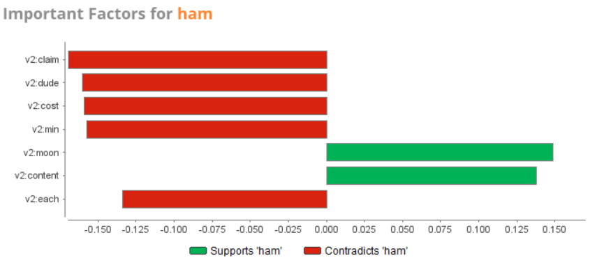
Gradient Boosted Trees

The Gradient Boosted Trees Operator trains a model by iteratively improving a single tree model. After each iteration step the Examples are reweighted based on their previous prediction. The final model is a weighted sum of all created models. Training parameters are optimized based on the gradient of the function described by the errors made.

In our data set the gradient boosted tree predicted that about 90% of given data is categorized as ham and 10% as spam. Important factors for contradicting ham included claim, dude, cost, min and each. Important factors for supporting ham included moon and content.

An interpretation of the results and their implications.

From the filtered dataset 12.65% of the messages were labeled as spam. We also made a word cloud to identify the frequently occurring word in both types of messages. The words were color coded by their type. Blue being ham and red being spam.

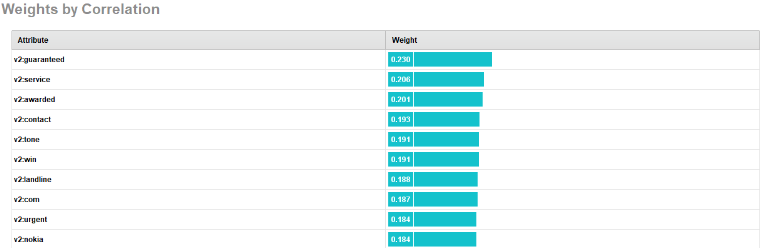
The most common words used by spam messages were usually selected to try and persuade the user. We generated a table of top 10 most recurring words and their weight, which indicated the frequency of use. The top 10 most recurring words ordering by their weight were guaranteed, service, awarded, contact, tone, win, landline, com, urgent and nokia.

A conclusion of the report.

In conclusion we used a new and interesting tool called RapidMiner for data analysis. Our dataset consisted of different SMS messages that were prelabeled. We used RapidMiners automated machine learning functionality with different algorithms to create the models.

After completing the task we thought that in the data cleaning set we could also have corrected all grammatical spelling mistakes. This would have helped us in a way that these words would be counted as one and not as two different words. It would have also been interesting to have even more data to work with since a lot of the SMS messages were very short and had no particular context.

Overall it  was interesting to see how easy the process was in reality and how the words in messages had either a positive or negative undertone to them. We will probably take that into account when sending messages in the future.

Testing dataset

After having a meeting with our lecturers we decided to make a testing dataset that included 500 rows of ham and 500 rows of spam.

We chose to generate the same models as before:
Naive Bayes
Generalized Linear Model
Fast Large Margin
Deep learning
Decision Tree
Random Forest
Gradient Boosted Trees

The accuracy of results was a lot smaller than before. This might be because the testing dataset we made was also significantly smaller than our actual dataset.

We ran the algorithms and got following grading results:
Naive Bayes – spam 7% , ham 93%
Generalized Linear Model – spam 56%, ham 44%
Fast Large Margin – spam 51%, ham 49%
Deep learning – spam 26%, ham 74%
Decision Tree – spam 30%, ham 70%
Random Forest – spam 43%, ham 57%
Gradient Boosted Trees – spam 48%, ham 52%

It was very interesting to see that the results from different algorithms varied a lot. The cause of this might be that a lot of spam SMS messages contained normal words that made it seem more like ham than spam. This shows us that from a short SMS message and much smaller dataset the obtained results might not be as trustable. A lot of the words from the messages were found in both ham and spam.

https://ifi7167socialcomputing.wordpress.com/2020/10/29/data-analysis-project-2-pick-up-a-dataset/

Social Network Analysis with Gephi

An introduction of the dataset

Our dataset was about users’ posts with their respective scores on different subreddits. The initial raw dataset contained fields like rawtime, total score of votes, reddit user information, subreddit that the content was posted on, number of comments and the username of the post creator. The data ranged from year 2008 to 2013 resulting in over 132 000 rows of data. Since there were no clear edges and nodes then we had to come up with a vision of our own and process the rows into a more meaningful dataset.

The goals of the analysis

The goal of the data analysis was to see which subreddit was the most popular in regards to the number of votes on a randomly selected month.

The methods that were used and their meaning

We began by analyzing the initial data we had available. During a brainstorming session we decided on just checking how users post scores related to different subreddits. For the processing we objected to using Python to process the initial csv file into two separate files. One was supposed to be the file with nodes with the fields: Id, username as Label and node_type either user or subreddit. The second one was a simple edges file with the target node and source node and the score of the connection as weight.

First of all we wanted to filter a selection from the dataset so that the end result would be a connection between the user and a subreddit with the score of the post.

We used the following Python script to achieve that:

After that we started creating the node and edge files. For the edges we wanted the cumulative post score of the user and subreddit combining all posts into one.

We used the following Python script:

Initially we didn’t have the singular month selection data and that resulted in too many nodes and connections, which Gephi couldn’t render too well and turned into abstract art.

After narrowing the data down to a single month 2012-09 then we got a simple node graph:

The selected month contributed to 17% of the total dataset, so we ended up with meaningful data.

Then we tested with different colors and layouts to try and make it pretty and understandable by adding labels and color coding the graph with modularity class.
For the clustering we used ForceAtlas 2 with the following parameters:

We also used giant component filtering to remove floating nodes that were not connected to the central cluster.

The results that were obtained

We calculated some overall network measures:

• Average degree: 1.11
• Average Path length: 3.3
• Network diameter: 10
• Modularity: 0.653
• Number of communities: 318

The low average degrees and path lengths suggest that the graph is loosely connected with some larger communities, since the degree of nodes portrays its connection count with other nodes. The largest interlinked connections results in a network diameter of 10 with 318 different communities.

Our network is of medium-high modularity which means that we have dense connections between nodes within modules but sparse connections between nodes in different modules.

Those were the most meaningful statistics for our particular graph. We couldn’t really get a meaningful centrality number due to the distribution of connections between nodes.

Final graph:

Five most popular subreddits and the number of votes:

1. Funny
   • number of votes: 6540
   • color on the graph: pink
2. Pics
   • number of votes: 2517
   • color on the graph: lime green
3. Gifs
   • number of votes: 1279
   • color on the graph: light blue
4. WTF
   • number of votes: 1248
   • color on the graph: orange
5. Aww
   • number of votes: 876
   • color on the graph: beige

An interpretation of the results and their implications

Looking at the final graph we can see clear clusters around popular subreddits. The most popular by a huge margin was /r/funny, to which a lot of other subreddits were linked. This proved to be quite interesting to see such “carrier” users connect different subreddits. Perhaps they were just reposting the same content on different platforms or perhaps they were just active users. This could be a point of further analysis in addition to taking in account the total score votes of the users in a more meaningful way.
It was also interesting to see smaller node trees around the main cluster, which showed passionate users only being active on those subreddits. Although they managed to be connected to the whole cluster by someone from the outside.

A conclusion of the report

In general this data analysis was really interesting due to the fact that our data was not premade and we had free reign over how we planned to use it. Looking back at the python code it could surely be improved and perhaps more meaningful data extracted from the initial dataset but overall the end results are satisfactory. Using Gephi raised new interesting questions about the data and possible ways of interpreting it.
We learned a lot about different data analysis techniques and practices, in addition to node cluster related parameters and equations.

https://ifi7167socialcomputing.wordpress.com/2020/09/17/social-computing-data-analysis-project1/

Assignment 4: Topics on Social Computing 3

Fake News, Hate Speech and Algorithmic Bias

Fake News Detection on Social Media: A Data Mining Perspective

• What constitutes a Fake News?

The term “Fake News” has no agreed definition. Most fake news are created with dishonest intention to mislead consumers. This study talked about fake news on traditional media and fake news on social media. The characterization for fake news on traditional media was explained with psychology foundations and social foundations. Fake news on social media characterization was explained as malicious accounts and echo chamber.

It is quite impossible to define fake news in terms of its medium so it is easier to focus on the nature of its content. When it comes to the psychological foundations of fake news, traditional fake news mainly targets consumers by exploiting their individual vulnerabilities. This study talked about two major factors which make consumers naturally vulnerable to fake news. First one being Na’ıve Realism and the second one Confirmation Bias. Social foundations of the fake news ecosystem also plays a big role in fake news on traditional media. Users are very likely to choose “socially safe”
options when consuming news information following the norms established in the community even if the news being shared is fake news. The study also said that fake news interactions can be modeled from an economic game theoretical perspective. It can almost be taken as a two-player strategy game between publisher and consumer. Fake news happen when the short-term utility dominates a publisher’s overall utility and psychology utility dominates the consumer’s overall utility, and an equilibrium is maintained.

All things mentioned about fake news on traditional media also apply to fake news on social media. When it comes to fake news on social media there are more possible ways to do it. One of wich is malicious accounts. Social media users don’t have to be real humans to function. Some of those users can actually be bots that are designed specifically with the purpose to spread fake news on social media. Social media also tends to have an echo chamber effect. Someone starts a fake news and there are people who will follow it. People will start making groups and forming a community that supports that fake news as if it was real.

• What are the strategies and open problems mentioned in the paper, related with the detection of Fake News in Online Social Media?

Methods for detection:

• Knowledge-based
• Style-based
• Stance-based
• Prpagation-based

Problems in detection:

• Users engagement with the news can make the fake news even more available and well known as it was before.

Automated Hate Speech Detection and the Problem of Offensive Language

• What constitutes Hate Speech?

Hate speech tends to be defined as speech that targets minority groups in a way that could promote violence or social disorder. This study defined hate speech as language that is used to expresses hatred towards a targeted group or is intended to be derogatory, to humiliate, or to insult the members of the group.

• What strategy did the authors propose to detect Hate Speech?

Fot the data they used a hate speech lexicon containing words and phrases identified by internet users as hate speech. After that they used a Twitter API to searche for tweets containing terms from the lexicon. They used tweets from 33,458 Twitter users resulting in a set of 85.4 million tweets. After that they took a random sample of 25K tweets that contained words from the lexicon. They had all of these tweets manually coded by workers who were asked to label each tweet as one of three categories: hate speech, offensive but not hate speech, or neither offensive nor hate speech. Only 5% of tweets were coded as hate speech. This study found that certain terms are particularly useful for distinguishing between hate speech and offensive language.

The Risk of Racial Bias in Hate Speech Detection

• What constitutes an Algorithmic Bias?

Algorithmic bias happens when there is a lack of training the data. This study showed that African Americans are up to two times more likely to be labelled as offensive compared to others when tweeting in their dialect.

• Mention some real-life consequences that can derive from the examples of Algorithmic Bias presented in the paper.

Hate speech primarily targets members of minority groups and can catalyze real-life violence towards them. The most common real-life consequence with racial biases can be the fact that black people are likely to receive longer sentences than white people who committed the same crime. There are so many other racial and ethnic biases that have been talked about in the media. When Google came out with image-identification algorithm in its Photos application identified black people as gorillas.

https://ifi7167socialcomputing.wordpress.com/2020/10/01/assignment-4-topics-on-social-computing-3/

Assignment 3: Topics on Social Computing 2

Crowdsourcing and Collective Intelligence

Reading Assignment

Give some examples of where “Games with a Purpose” have been used and why.

“Games with a Purpose” have been used in areas as diverse as security, computer vision, Internet accessibility, adult content filtering, and Internet search. 

This article gave four game examples that fit into this kind of criteria. First two games that were talked about were ESP Game and Peekaboom. Two additional games that they mentioned were still under development. First game was called Phetch and the second one Verbosity.

All of these games demonstrate that people can solve problems that computers can’t yet solve. People playing video games have the potential to simultaneously solve large-scale problems without even realizing it.

ESP Game is a two person game where the goal is to guess what label your partner would give to the image. This game can determine what image is shown on the picture but it can not give away any location information that would be necessary for training and testing computer vision algorithms. This game managed to collect over 10 million image labels after first being deployed on 25 October 2003. This result only took a few months so if this game would be hosted on a major site then all of the images on the Web would be labeled in a few weeks.

Peekaboom game concentrates more on the location aspect. In this game two players are assigned the roles of “Peek” and “Boom”. Peeks goal is to guess the associated word while Boom slowly reveals the image. This game also collects location data by identifying which pixels belong to which object in the image. 

The purpose of these kinds of games is that the players feel entertained while solving problems.

Explain how the ESP games motivate people to “think like each other”.

In order to win the game two players must write the same words. When you can guess what word the other player is going to write you win and a new image appears. So in order to win you must start to think like each other. What word would the other player use to describe this picture? 

The article says “The only thing partners have in common [in the ESP game] is an image they can both see.” I would say that this is not the whole truth. There is one important other thing that players share, otherwise the game would not work. What is it and why is it important?

No game would ever work without the motivation to win. Players must think like each other and write the same words in order to win. They can not just write down any words but they truly have to start thinking like each other. They have to know what the other player will do before they actually do it. I think that sums up why we need people for that and not computers.

https://ifi7167socialcomputing.wordpress.com/2020/09/20/assignment-3-topics-on-social-computing-2/

Assignment 1: Pick a Case Analysis Project

Kärol-Milaine Jürgenson
Risto Leesmäe

Wikipedia: The most successful encyclopedia in the world

Wikipedia is in short an open-source encyclopedia that is created and edited by its readers. After its creation in 2001, it has grown enormously, attracting 1.5 billion unique visitors monthly. It has more than 54 million articles spanning over 300 languages. By this point you may be asking, how this platform manages to operate.

Well Wikipedia is supported by five fundamental principles:

• Is an encyclopedia
• Written from a neutral point of view
• Free content that anyone can use, edit, and distribute
• Editors should treat each other with respect and civility
• Has no firm rules

All this means that Wikipedia is continually created and updated, with articles on new events appearing within minutes, rather than months or years. Currently around 130 000 contributors per month who are actively taking part in keeping Wikipedia’s content up to date and relevant. While you read this, Wikipedia develops at a rate of over 1.9 edits per second. Currently, the English Wikipedia includes 6,156,460 articles and it averages 1,500 new articles per day. For comparison Estonian Wikipedia includes 211 829 articles and it averages 473 co-authors per month.

Because everybody can help improve it, Wikipedia has become more comprehensive than any other encyclopedia, also resulting in huge growth of the platform. The number of articles in Wikipedia is increasing by over 17,000 a month. The number of articles added to Wikipedia every month reached its maximum in 2006, at over 50,000 new articles a month, and has been slowly but steadily declining since then.

This seems great in theory but won’t the users be able to just add false information to the encyclopedia? Thankfully this has been addressed and bots in addition to users try to minify vandalism. Vandalism includes any addition, removal, or modification that is humorous, nonsensical, a hoax, or otherwise degrading. Vandalism is easy to commit on Wikipedia because anyone can edit the site. This is countered by the pages revision history, which shows the following:

• Comparison to other revisions
• Timestamp of the change
• User who made the change, including the users information
• Information about the change
• Undo functionality to roll back to previous revisions

There are many semi-protected pages where new and unregistered people can not edit. More than one thousand pages are deleted from Wikipedia each day. 

The most well-known “bot” that fights vandalism on Wikipedia pages is ClueBot NG. The bot was created by Wikipedia users Christopher Breneman and Cobi Carter in 2010. The bot uses machine learning and Bayesian statistics to determine if an edit is vandalism.

In addition to using bots there is also a title blacklist and spam blacklist that prevents external link spamming. Certain images have also been blacklisted from Wikipedia, since they have been deemed potentially offensive. All of these images are accessible for everyone to see here.

Wikipedia editors may face numerous restrictions on freedom of speech, including various types of sanctions. Many articles are deleted via the proposed deletion and speedy deletion processes while others are deleted according to subjective criteria such as lack of significance or lack of notability.

Users are able to communicate and discuss ideas with others on the platform. They are given special awards for their contribution on the site and all their previous revisions are available for everyone to see. This in turn creates a status and ranking system, to further verify the credibility of the users changes.

Wikipedia is an amazing free platform where everyone can freely share their knowledge. The data is supplied by a vast userbase who contribute and moderate the sites content without any obligations. This results in fast creation of articles and correction of misinformation. In my opinion Wikipedia has played a huge role in our modern society, what do you think?

References:

Stvilia, Besiki, et al. “Information quality discussions in Wikipedia.” Proceedings of the 2005 international conference on knowledge management. 2005. http://citeseerx.ist.psu.edu/viewdoc/download?doi=10.1.1.84.3912&rep=rep1&type=pdf

Priedhorsky, Reid, et al. “Creating, destroying, and restoring value in Wikipedia.” Proceedings of the 2007 international ACM conference on Supporting group work. 2007. Click to access group282-priedhorsky.pdf

Kittur, Aniket, and Robert E. Kraut. “Harnessing the wisdom of crowds in wikipedia: quality through coordination.” Proceedings of the 2008 ACM conference on Computer supported cooperative work. 2008. https://dl.acm.org/doi/pdf/10.1145/1460563.1460572?casa_token=z5tetJSH1VkAAAAA:6ABdxbb8e1tTgaOF_1fM-1M-IabC9vpeAcnxKwyCeuzlosIZtb9zwh5MI8hmv2GXlcGKLTPL0cvNlw

Erickson, Thomas: Social Computing, chapter 4.5 Social Computing as a system: Wikipedia In: Soegaard, Mads and Dam, Rikke Friis (eds.). “The Encyclopedia of Human-Computer Interaction, 2nd Ed.”. Aarhus, Denmark: The Interaction Design Foundation. 2013. https://www.interaction-design.org/literature/book/the-encyclopedia-of-human-computer-interaction-2nd-ed/social-computing#heading_Social_Computing_as_a_system:_Wikipedia_html_pages_100753

Jim Giles. “Internet encyclopaedias go head to head.” Nature; Dec 15, 2005; pg. 900 https://www.nature.com/articles/438900a

https://ifi7167socialcomputing.wordpress.com/2016/04/14/assignment-2-pick-a-case-analysis-project/

Assignment 2: Topics on Social Computing 1

Tie strength in question answer on social network sites

How do the authors define strong and weak ties, and how did they measure the strength of a tie in Social Network Sites?

The primary idea behind tie strength is that, amongst our network of friends, we have friends with whom we are close and friends who are less close, acquaintances or weak ties.

The process for generating tie strength in this study was drawn directly from Gilbert and Karahalios’ study made in 2009.

Work by Gilbert and Karahalios looked at Granovetter’s denotation of strong and weak ties within real-life offline social networks and found a series of features that can effectively predict tie strength between friends in an online social network.

In this study they used Gilbert and Karahalios method by predicting tie strength using features and content from Facebook. The data required for generating tie strength was gained from Facebook’s Download Your Data feature. This allowed them to capture all of the communication between the participants and their friends. Participants were asked to download their data before the study and before asking a question for their study, so that participation in the study would not affect generated tie strengths.

Predictive variables used were:

• Days since last communication
• Days since first communication
• Words exchanged
• Mean tie strength of mutual friends
• Positive emotion words
• Intimacy words

Since they used a simplified version of Gilbert’s model, they attempted to calibrate their results by asking participants a question in the survey portion about how much they valued information from each of the answerers in general. This got them to a result that the correlation was statistically significant. Several months after the initial study, they also asked participants to rate the tie strength of a selection of their friends as well. This also resulted in a strong correlation.

What could be the reasons that more helpful answers come from weak ties?

Weak ties are valuable in that they can tie together different network groups. Weak ties are more likely to link different groups together by a bridge and so can provide new information from one group to another. Relationships with your weak ties should be maintained and cultivated, combining networks together to encourage information flow between the different parts of your networks. Weak ties are most crucial in the job searching process. Most people find jobs through contacts they see either rarely or occasionally. Same goes about any information that your network does not have knowledge about. That is the reason why more helpful answers might come from weak ties. Weak ties have information that your network might not have.

What could be the reasons that more helpful answers come from strong ties?

A strong tie is someone who you know well and with whom information runs freely. Strong ties are valuable in that they tie together groups that share specific things in common. When it comes to answering questions friends-of friends ought to be more effective than strangers in answering questions. Morris et al found that, in a small study, many participants’ questions were answered by friends they rated as close. Strong ties may contribute slightly more to the overall knowledge gained by participants, and share less information the participant already knew. Since close ties give us more information about things that we already have some knowledge about it makes us trust it more. People generally acknowledge information given from close friends more than from people that we barely know.

As participants were especially looking for reliable information, how could reliability of the information source be measured in Social Networks?

Reliability had no statistically significant correlation with tie strength in this study, though it seems to be a big factor in determining answer quality for many participants. Different participants had different reasoning for reliability. On the other hand, the correlation between how much the answer contributed to participants’ overall knowledge and how trustworthy the answer was significant, and predicted 66% of the overall knowledge gained.

For one participant reliable information meant that the person answering didn’t just recommend something but also gave reasons from their experiences and pointed out other reliable sources.

More participants found that reliability has to do with the person. If they know that the person answering their questions has knowledge about the topic then they tend to trust their answer more than others.

Both strong and weak ties provided decision making information.

https://ifi7167socialcomputing.wordpress.com/2016/04/14/assignment-1-topics-on-social-computing-1